Jupyter Notebooks

Jupyter Notebooks are an open-source web application that allows you to create and share documents that contain live code, equations, visualizations, and narrative text. They are widely used in data science, machine learning, and scientific computing for data cleaning and transformation, numerical simulation, statistical modeling, data visualization, and machine learning.

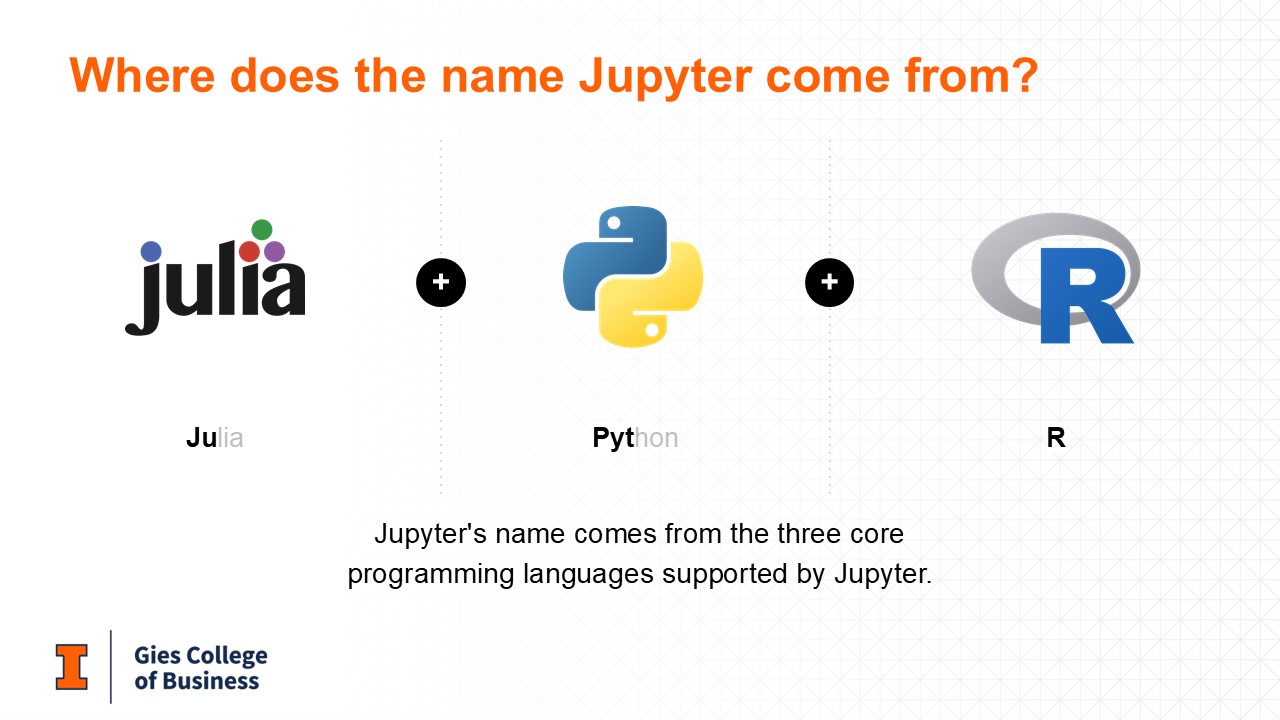
The name “Jupyter” is a combination of “Julia”, “Python”, and “R”, which are three programming languages commonly used in data science. The name also pays homage to Galileo’s notebooks, as Jupiter is the largest planet in our solar system and was named after the Roman god Jupiter.

🚀 Why Use Jupyter Notebooks?¶

• Interactive Coding: You can write and execute code in small chunks (cells), making it easier to test and debug.
• Rich Media: You can include images, videos, and interactive visualizations alongside your code.
• Documentation: You can use Markdown to create well-documented notebooks that explain your code and findings.
• Reproducibility: Notebooks can be shared and rerun by others, ensuring that your analyses can be reproduced.
• Integration: Jupyter supports many programming languages, including Python, R, and Julia.

💻 Installing and Running Jupyter Notebooks¶

There are multiple ways to run Jupyter Notebooks:

1. JupyterLab Desktop App (recommended for this course): JupyterLab is the next-generation user interface for Jupyter Notebooks. It provides a more flexible and powerful environment for working with notebooks, code, and data. You can download the JupyterLab desktop app from here.

2. Anaconda Distribution (Local Installation via Anaconda): Anaconda is a popular distribution of Python and R for scientific computing and data science. It comes with Jupyter Notebooks pre-installed. You can download Anaconda from here.

3. JupyterLab (Local Installation via pip): JupyterLab is the next-generation user interface for Jupyter Notebooks. It provides a more flexible and powerful environment for working with notebooks, code, and data. You can install it using pip:

   pip install jupyterlab

   Then, you can start JupyterLab by running:

   jupyter lab

4. Visual Studio Code (VS Code): VS Code is a popular code editor that supports Jupyter Notebooks through an extension. You can install the “Jupyter” extension from the VS Code marketplace. More information can be found here.

5. Google Colab: Google Colab is a free cloud-based service that allows you to run Jupyter Notebooks without any local installation. You can access it at colab.research.google.com. It provides free access to GPUs and TPUs, making it suitable for machine learning tasks. However, this may be an inconvenient option for this course, as you will need to upload and download files frequently.

🔄 Jupyter’s Read-Eval-Print Loop (REPL)¶

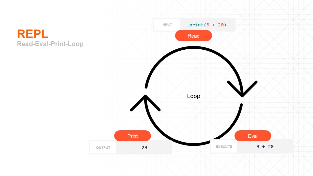
The Jupyter Notebook interface operates as a Read-Eval-Print Loop (REPL). REPL is the fundamental loop behind interactive programming environments. It consists of three main steps:

1. Read: The system takes in user input (e.g., print(3 + 20)).
2. Eval: The input is evaluated by the interpreter. In this case, it executes the expression 3 + 20.
3. Print: The result of evaluation (23) is printed back to the user.

This is why when you open a Python shell, you can type a command, see the result immediately, and continue typing more commands interactively — it’s the REPL cycle at work.

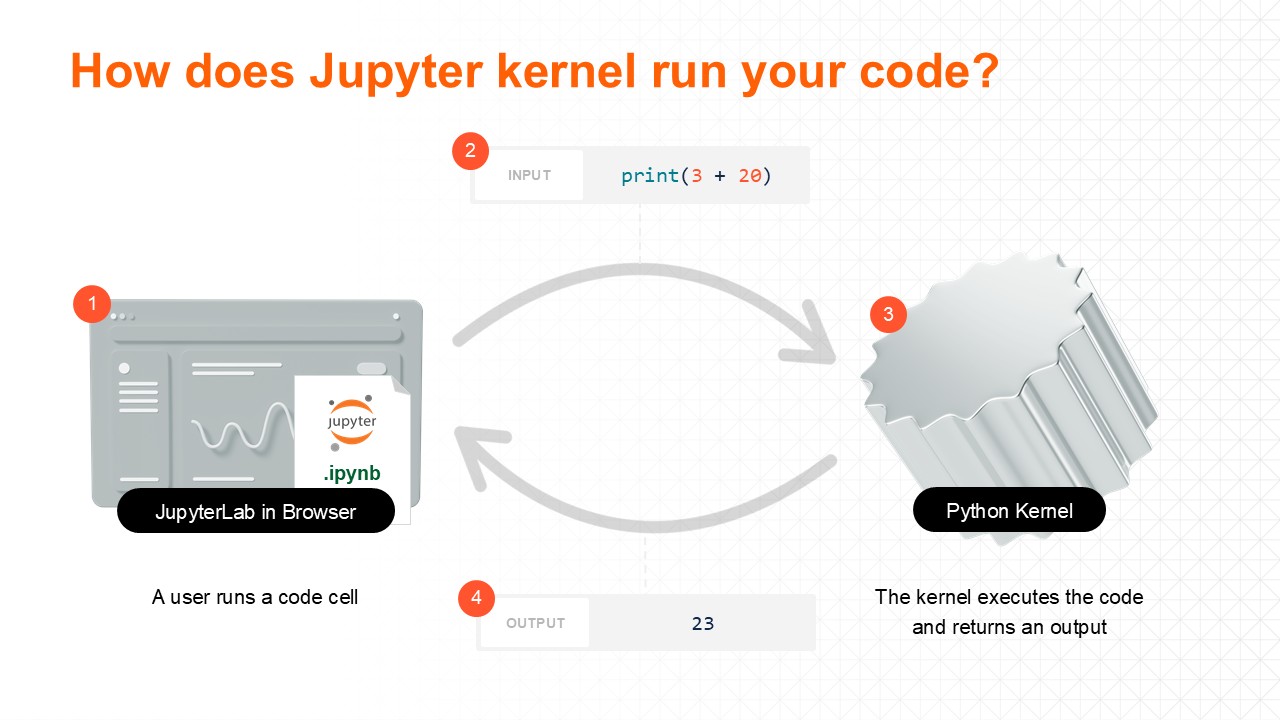
The underlying process for a Jupyter Notebook environment is REPL-based — just separated into a client (browser interface) and a backend (kernel).

1. JupyterLab in Browser: A user runs a code cell inside the Jupyter Notebook (.ipynb).
2. Input: The content of the cell (e.g., print(3 + 20)) is sent to the backend.
3. Python Kernel: The kernel executes the code, just like the “Eval” step in REPL.
4. Output: The kernel sends the result (23) back to JupyterLab, which displays it under the code cell.

🧠 Maintaining State with the Kernel¶

The kernel maintains the state of the notebook, including variables, functions, and imports. This means that you can run code cells in any order, and the state will persist until you restart the kernel or close the notebook.