▶️ Import pandas and numpy.
import pandas as pd
import numpy as np
▶️ Create a new DataFrame named df_emp.
df_emp = pd.DataFrame(
    {
        "emp_id": [30, 40, 10, 20],
        "name": ["Toby", "Jim", "Pam", "Kelly"],
        "dept": ["HR", "Sales", "Sales", "Customer Service"],
        "office_phone": ["(217)123-4500", np.nan, np.nan, "(217)987-6600"],
        "start_date": ["2017-05-01", "2018-02-01", "2020-08-01", "2019-12-01"],
        "salary": [202000, 185000, 240000, 160500],
    }
)

# Create a backup copy of the original DataFrame
df_emp_backup = df_emp.copy()

df_emp▶️ Run df_emp.info() for a summary of the DataFrame, including the data types of each column and the number of non-null entries.
df_emp.info()<class 'pandas.core.frame.DataFrame'>
RangeIndex: 4 entries, 0 to 3
Data columns (total 6 columns):
# Column Non-Null Count Dtype
--- ------ -------------- -----
0 emp_id 4 non-null int64
1 name 4 non-null object
2 dept 4 non-null object
3 office_phone 2 non-null object
4 start_date 4 non-null object
5 salary 4 non-null int64
dtypes: int64(2), object(4)
memory usage: 324.0+ bytes
🗓️ Working with Datetime Values
Datetime values are common in datasets. They can represent dates, times, or both. Pandas provides powerful tools to work with datetime data.
A few common datetime formats include:
YYYY-MM-DD(e.g.,2021-03-15)MM/DD/YYYY(e.g.,03/15/2021)DD-Mon-YYYY(e.g.,15-Mar-2021)YYYYMMDD(e.g.,20210315)
When you read a CSV file, pandas does not automatically recognize datetime columns.
▶️ You can verify this by checking the data type of the "start_date" column.
display(df_emp["start_date"])
print(str(df_emp["start_date"].dtype))  # Check the data type of the "start_date" column
0 2017-05-01
1 2018-02-01
2 2020-08-01
3 2019-12-01
Name: start_date, dtype: objectobject
The "start_date" column is currently of type object, which means it is treated as a string.
To use datetime functionalities, we need to convert this column to a datetime type. There are two ways to convert a column to datetime:
During CSV Import: Use the
parse_datesparameter inpd.read_csv().df = pd.read_csv('data.csv', parse_dates=['date_column'])After CSV Import: Use
pd.to_datetime()to convert a column.df['date_column'] = pd.to_datetime(df['date_column'])
🎯 Example: Parse the start_date column as datetime
We will create a new column "start_date_parsed" that contains the parsed datetime values.
df_emp["start_date_parsed"] = pd.to_datetime(df_emp["start_date"])

df_emp▶️ Run str(df_emp["start_date_parsed"].dtype) to check the data type of the new "start_date_parsed" column.
str(df_emp["start_date_parsed"].dtype)'datetime64[ns]'▶️ Drop the "start_date" column and rename "start_date_parsed" to "start_date".
This effectively replaces the original string column with the new datetime column.
df_emp.drop(columns=["start_date"], inplace=True)
df_emp.rename(columns={"start_date_parsed": "start_date"}, inplace=True)

df_emp▶️ Check the data types of the columns to confirm the change.
df_emp.dtypesemp_id int64
name object
dept object
office_phone object
salary int64
start_date datetime64[ns]
dtype: objectNow the "start_date" column is of type datetime64[ns], which allows us to perform datetime operations on it.
🔢 Extract Date Components
We can easily extract components like year, month, and day from datetime columns using the .dt accessor.
df['year'] = df['date_column'].dt.year
df['month'] = df['date_column'].dt.month
df['day'] = df['date_column'].dt.day
df['weekday'] = df['date_column'].dt.weekday     # e.g., 0=Monday, 6=Sunday
df['weekday'] = df['date_column'].dt.day_name()  # e.g., 'Monday'
We can also extract more specific components like hour, minute, and second if the datetime includes time.
df['hour'] = df['date_column'].dt.hour
df['minute'] = df['date_column'].dt.minute
df['second'] = df['date_column'].dt.second
▶️ Extract the year, month, and day from the "start_date" column into new columns "start_year", "start_month", and "start_day".
df_emp["start_year"] = df_emp["start_date"].dt.year
df_emp["start_month"] = df_emp["start_date"].dt.month
df_emp["start_day"] = df_emp["start_date"].dt.day

df_empIf you’re working with quarterly or weekly data, you can extract those components as well.
df['quarter'] = df['date_column'].dt.quarter          # e.g., 1, 2, 3, 4
df['week'] = df['date_column'].dt.isocalendar().week  # e.g., 1-52
▶️ Extract the quarter and week from the "start_date" column. This time, we will not create new columns but will display the results directly.
df_emp["start_date"].dt.quarter0 2
1 1
2 3
3 4
Name: start_date, dtype: int32df_emp["start_date"].dt.isocalendar().week0 18
1 5
2 31
3 48
Name: week, dtype: UInt32🔬 Grouping and Aggregating Data with Pandas
A common task in data analysis is to summarize data by certain criteria, such as calculating averages or totals for different groups within the data.
In the employees dataset, you might want to find out the average salary by department, or the total number of employees hired each year.
Pandas allows you to use the groupby() method to group data by one or more columns, and then apply aggregation functions like mean(), sum(), count(), etc.
This follows the split-apply-combine pattern used in many data analysis workflows.
The split-apply-combine consists of three steps:
Split: Divide the data into groups based on one or more keys (columns).
Apply: Apply a function (e.g., aggregation, transformation) to each group.
Combine: Combine the results back into a DataFrame.
To illustrate the split-apply-combine process, we will create a new DataFrame.
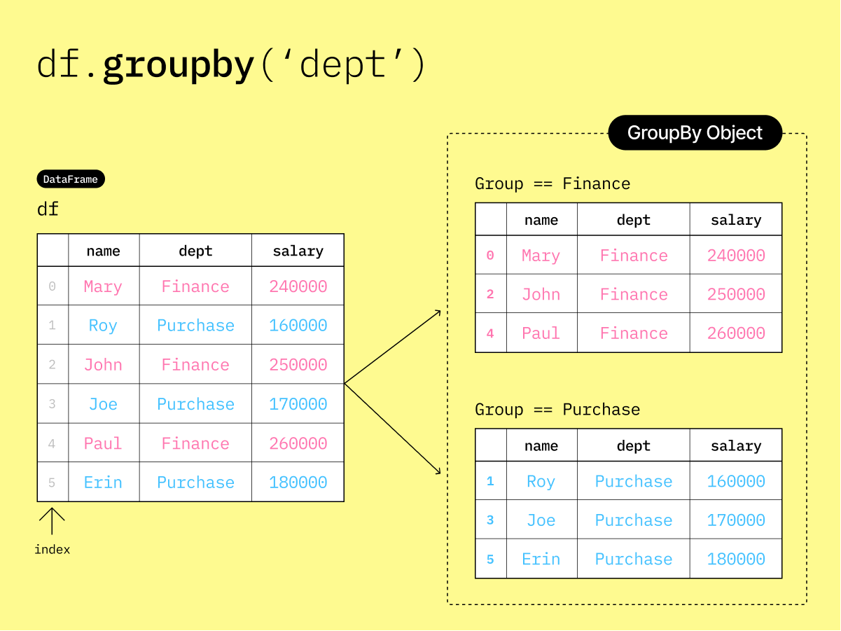
▶️ Create a new DataFrame named df.
df = pd.DataFrame(
    {
        "name": ["Mary", "Roy", "John", "Joe", "Paul", "Erin"],
        "dept": ["Finance", "Purchase", "Finance", "Purchase", "Finance", "Purchase"],
        "salary": [240000, 160000, 250000, 170000, 260000, 180000],
    }
)

df▶️ Group the DataFrame df by the "dept" column without applying any aggregation function.
This creates a DataFrameGroupBy object, which represents the grouped data but does not perform any computations yet.
df.groupby("dept")<pandas.core.groupby.generic.DataFrameGroupBy object at 0x0000023972A07EF0>This diagram illustrates the DataFrameGroupBy object created by df.groupby('dept').
🗂️ Aggregate a DataFrameGroupBy object
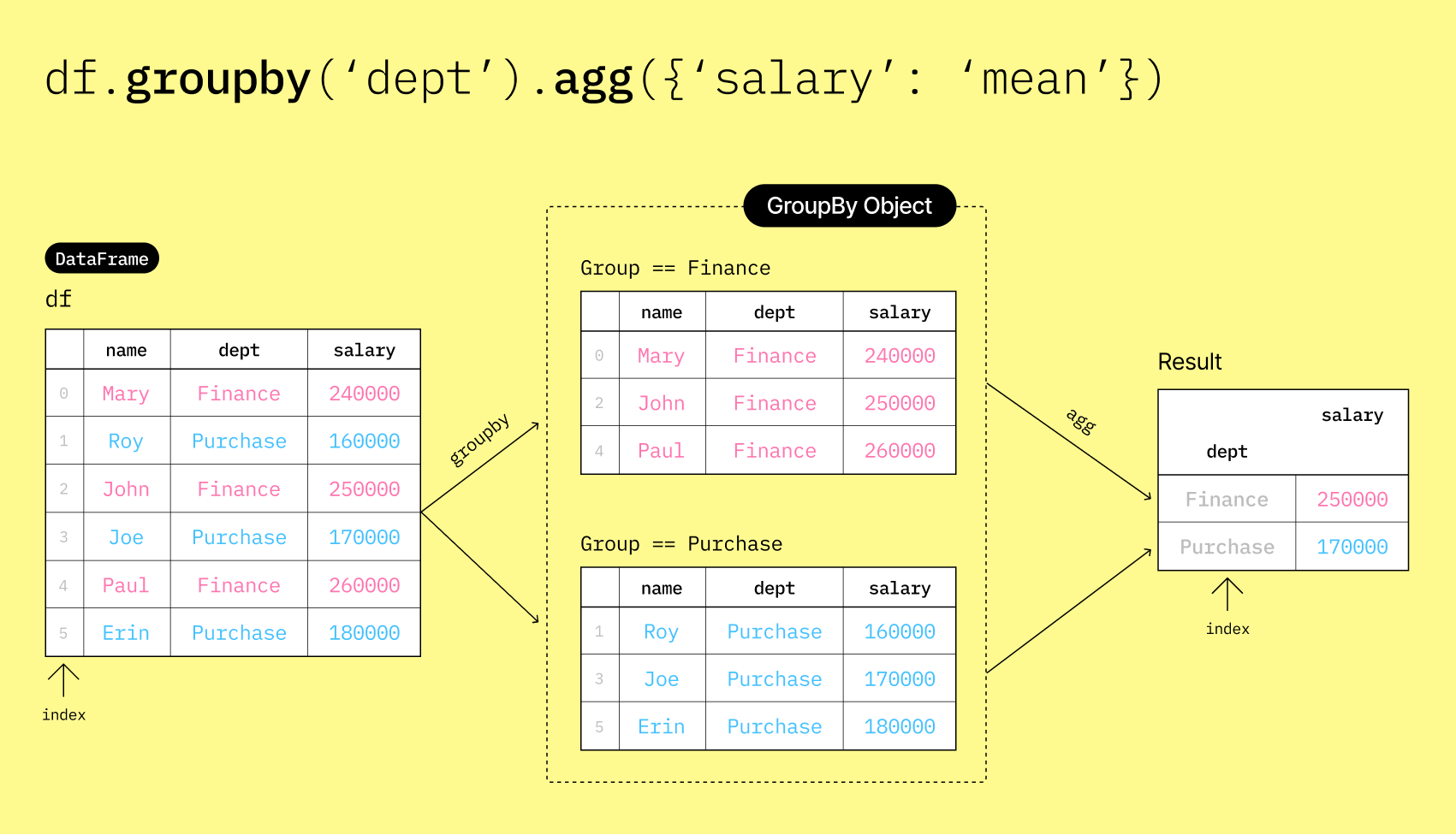
▶️ Group the DataFrame df by the "dept" column and calculate the mean salary for each department using the agg() method.
df_salary_by_dept = df.groupby("dept").agg({"salary": "mean"})

df_salary_by_deptThe result is a new DataFrame that shows the average salary for each department.
Columns and Index (Row Labels) in Aggregated DataFrames
▶️ Check the columns of the resulting DataFrame.
print(df_salary_by_dept.columns)Index(['salary'], dtype='object')
Although the output shows two columns (dept and salary), printing the columns only show the salary column. This is because the output of df_salary_by_dept uses the "dept" column as the index.
An index in pandas is a special column that uniquely identifies each row in a DataFrame. It is not considered a regular column and is not included in the columns attribute. When you group by a column, that column is set as the index of the resulting DataFrame by default.
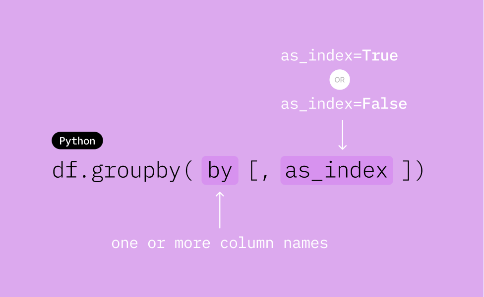
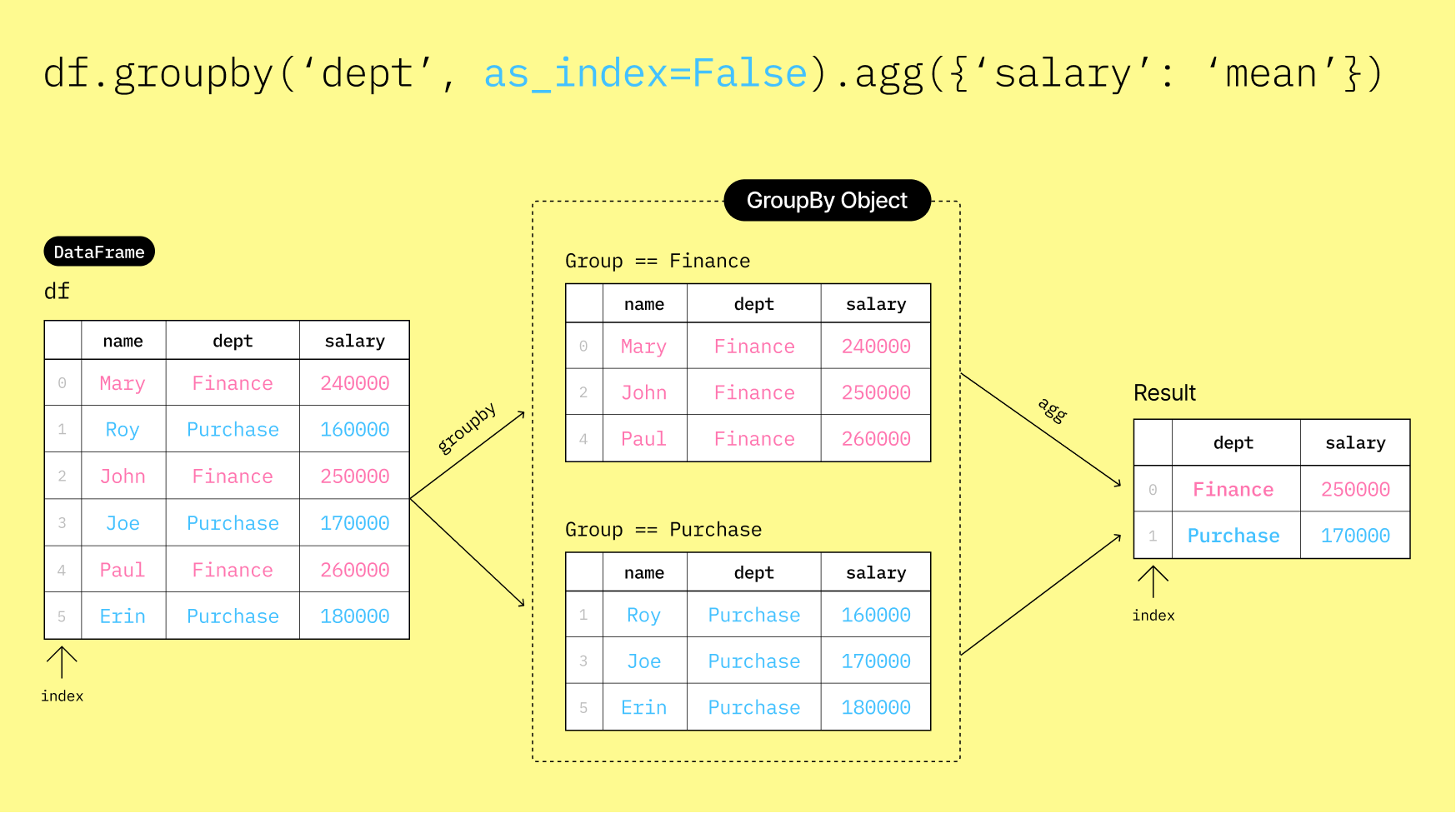
📂 Aggregate a DataFrameGroupBy object with optional index=False
▶️ Specify as_index=False in the groupby() method to keep the grouping column as a regular column instead of setting it as the index.
df_salary_by_dept2 = df.groupby("dept", as_index=False).agg({"salary": "mean"})

df_salary_by_dept2▶️ Check the columns of the resulting DataFrame.
print(df_salary_by_dept2.columns)Index(['dept', 'salary'], dtype='object')
Since we specified as_index=False, the "dept" column is retained as a regular column in the resulting DataFrame. Now, printing the columns shows both dept and salary.
➗ Calculate multiple statistics
▶️ Instead of calculating just the mean salary, you can calculate multiple statistics at once by passing a list of aggregation functions to the agg() method’s dictionary.
df_salary_by_dept3 = df.groupby("dept", as_index=False).agg(
    {"salary": ["min", "max", "mean", "sum", "count", "std"]}
)

df_salary_by_dept3▶️ Check the columns of the resulting DataFrame.
print(df_salary_by_dept3.columns)MultiIndex([( 'dept', ''),
('salary', 'min'),
('salary', 'max'),
('salary', 'mean'),
('salary', 'sum'),
('salary', 'count'),
('salary', 'std')],
)
Notice that the columns now have a hierarchical structure (a MultiIndex) because we applied multiple aggregation functions to the "salary" column. The first level is the original column name (salary), and the second level contains the names of the aggregation functions (min, max, mean, sum, count, std).
🪄 Flatten multi-level index columns
It is perfectly fine to work with multi-level columns, but sometimes you may want to flatten them for easier access. You can manually assign the column names after aggregation to flatten the columns.
df_salary_by_dept4 = df.groupby('dept', as_index=False).agg({'salary': ['min', 'max', 'mean', 'sum', 'count', 'std']})
display(df_salary_by_dept4)
print('Columns before (multi-level, not flat):')
print(df_salary_by_dept4.columns)
# manually assign column names
df_salary_by_dept4.columns = ['dept', 'min_salary', 'max_salary', 'mean_salary', 'total_salary', 'num_employees', 'std_dev']
display(df_salary_by_dept4)
print('Columns after (flat-level):')
print(df_salary_by_dept4.columns)▶️ Copy the provided code to the code cell below and run it.
df_salary_by_dept4 = df.groupby("dept", as_index=False).agg(
{"salary": ["min", "max", "mean", "sum", "count", "std"]}
)
df_salary_by_dept4▶️ Check the columns of the DataFrame before flattening.
print("Columns before flattening:")
df_salary_by_dept4.columnsColumns before flattening:
MultiIndex([(  'dept',      ''),
            ('salary',   'min'),
            ('salary',   'max'),
            ('salary',  'mean'),
            ('salary',   'sum'),
            ('salary', 'count'),
            ('salary',   'std')],
)▶️ Flatten the columns by manually assigning new column names.
df_salary_by_dept4.columns = [
    "dept",
    "min_salary",
    "max_salary",
    "mean_salary",
    "total_salary",
    "num_employees",
    "std_dev",
]

df_salary_by_dept4▶️ Check the columns of the DataFrame after flattening.
print("Columns after flattening:")

df_salary_by_dept4.columns
Columns after flattening:
Index(['dept', 'min_salary', 'max_salary', 'mean_salary', 'total_salary',
       'num_employees', 'std_dev'],
      dtype='object')
📞 Examples Using Bank Marketing Calls Data
Let’s apply what we’ve learned to a real-world dataset. We’ll use a dataset related to direct marketing campaigns (phone calls) of a banking institution.
Data Source: [Moro et al., 2014] S. Moro, P. Cortez and P. Rita. A Data-Driven Approach to Predict the Success of Bank Telemarketing. Decision Support Systems, Elsevier, 62:22-31, June 2014
📖 Data Dictionary
| Column Name | Type | Description |
|---|---|---|
age | Numeric | Age |
job | Categorical | admin.', ‘blue-collar’, ‘entrepreneur’, ‘housemaid’, ‘management’, ‘retired’, ‘self-employed’, ‘services’, ‘student’, ‘technician’, ‘unemployed’, ‘unknown’ |
marital | Categorical | single’, ‘married’, ‘divorced’, ‘unknown’ |
education | Categorical | basic.4y’, ‘basic.6y’, ‘basic.9y’, ‘high.school’, ‘illiterate’, ‘professional.course’, ‘university.degree’, ‘unknown’ |
contact_type | Categorical | cellular’, ‘telephone’ |
num_contacts | Numeric | Number of contacts performed during this campaign for this client |
prev_outcome | Categorical | Outcome of the previous marketing campaign - ‘failure’, ‘nonexistent’, ‘success’ |
place_deposit | Numeric | Did the client subscribe to a term deposit? This column indicates whether the campaign was successful (1) or not (0) for each client. |
Analyze the dataset to discover relationships between personal factors and marketing campaign result of each individual.
place_deposit column indicates whether a marketing campaign was successful.
✅ If
1, the individual has placed a deposit within the bank. This is considered a successful campaign.🚫 If
0, the individual has not placed a deposit within the bank. This is considered an unsuccessful campaign.
▶️ Load the bank marketing calls dataset into a new DataFrame named df_bank.
df_bank = pd.read_csv(
    "https://github.com/bdi475/datasets/blob/main/bank-direct-marketing.csv?raw=true"
)
df_bank🎯 Example: Marketing success rate by marital status
Find out which marital status group has the highest marketing success rate.
▶️ Group the DataFrame by the "marital" column and calculate the mean of the "place_deposit" column for each group.
df_by_marital = df_bank.groupby("marital", as_index=False).agg(
    {"place_deposit": "mean"}
)
df_by_marital


df_by_marital▶️ Rename the "place_deposit" column to "success_rate".
df_by_marital.rename(columns={"place_deposit": "success_rate"}, inplace=True)

df_by_marital▶️ Sort the resulting DataFrame by "success_rate" in descending order to see which marital status has the highest success rate.
df_by_marital.sort_values("success_rate", ascending=False, inplace=True)

df_by_marital🎯 Example: Marketing success rate by job
Find out which job category has the highest marketing success rate.
df_by_job = df_bank.groupby("job", as_index=False).agg({"place_deposit": "mean"})
df_by_job.rename(columns={"place_deposit": "success_rate"}, inplace=True)
df_by_job.sort_values("success_rate", ascending=False, inplace=True)

df_by_job🎯 Example: Marketing success rate by contact type with count
▶️ Group the df_bank DataFrame by the "contact_type" column and calculate both the mean of the "place_deposit" column (to get the success rate) and the count of records for each contact type. Use as_index=False to keep "contact_type" as a regular column.
df_by_contact_type = df_bank.groupby("contact_type", as_index=False).agg(
    {"place_deposit": ["count", "mean"]}
)

# flatten columns
df_by_contact_type.columns = ["contact_type", "count", "success_rate"]

# sort by success_rate in descending order
df_by_contact_type.sort_values("success_rate", ascending=False, inplace=True)

df_by_contact_type🎯 Example: Marketing success rate by marital status and contact type
You might want to see how the success rate varies not just by marital status, but also by the type of contact method used (cellular or telephone). This will help the bank understand which combinations of marital status and contact type are most effective.
To group by both marital status and contact type, you can pass a list of the two columns to the groupby() method.
▶️ Group the data by both "marital" status and "contact_type" to see how the success rate varies across these two dimensions.
df_by_type_and_marital = df_bank.groupby(
    ["marital", "contact_type"], as_index=False
).agg({"place_deposit": "mean"})
df_by_type_and_marital.rename(columns={"place_deposit": "success_rate"}, inplace=True)
df_by_type_and_marital.sort_values("success_rate", ascending=False, inplace=True)

df_by_type_and_marital🧲 Merging Two DataFrames (Joins)
In data analysis, your data is often spread across multiple tables or files. To get a complete picture, you need to combine these tables based on common information. In pandas, this operation is called a “merge,” which is analogous to “joins” in SQL.
The pd.merge() function is the primary tool for this task. It allows you to combine DataFrames in several ways, depending on what you want to do with records that don’t have matches in the other table.
To demonstrate how merging works, we’ll work a record of transactions from a small food stand selling only two items - sweetcorns 🌽 and beers 🍺. The tables associated with the food stand’s transactions are shown below.
Products (df_products)
| product_id | product_name | price |
|---|---|---|
| SC | Sweetcorn | 3.0 |
| CB | Beer | 5.0 |
Transactions (df_transactions)
| transaction_id | product_id |
|---|---|
| 1 | SC |
| 2 | SC |
| 3 | CB |
| 4 | SC |
| 5 | SC |
| 6 | SC |
| 7 | CB |
| 8 | SC |
| 9 | CB |
| 10 | SC |
▶️ Create the two tables as DataFrames.
df_products = pd.DataFrame(
    {
        "product_id": ["SC", "CB"],
        "product_name": ["Sweetcorn", "Beer"],
        "price": [3.0, 5.0],
    }
)

df_productsdf_transactions = pd.DataFrame(
{
"transaction_id": [1, 2, 3, 4, 5, 6, 7, 8, 9, 10],
"product_id": ["SC", "SC", "CB", "SC", "SC", "SC", "CB", "SC", "CB", "SC"],
}
)
df_transactions🎯 Example: Merge products into transactions
df_merged = pd.merge(
    left=df_transactions, right=df_products, on="product_id", how="left"
)

df_merged🎯 Example: Find total sales by product
df_sales_by_product = df_merged.groupby("product_id", as_index=False).agg(
    {"price": "sum"}
)

df_sales_by_productWhile the output is useful, it would be more informative to see the product names alongside their total sales. We can achieve this by grouping the merged DataFrame by both "product_id" and "product_name".
df_sales_by_id_name = df_merged.groupby(
    ["product_id", "product_name"], as_index=False
).agg({"price": "sum"})

df_sales_by_id_name📐 Types of Merges (Joins)
There are several types of joins you can perform when merging DataFrames. The most common types are:
Inner: Returns only the rows with keys that are present in both DataFrames.
Left: Returns all rows from the left DataFrame, and the matched rows from the right DataFrame. If there is no match, the result is
NaNon the right side.Right: Returns all rows from the right DataFrame, and the matched rows from the left DataFrame. If there is no match, the result is
NaNon the left side. This is the opposite of a left join.Outer: Returns all rows from both DataFrames.
👩🏽💻 Example Scenario: Employees and Laptops
To demonstrate the different types of joins, we will use a scenario involving employees and company laptops.
Assume we have three employees and four laptops. Each employee may or may not have a laptop assigned to them.

Assume that:
Jasper is assigned laptop A.
Gary is assigned laptop B.
Sally is not assigned a laptop. She works remotely and uses her own device.
Laptops C and D are unused and unassigned.
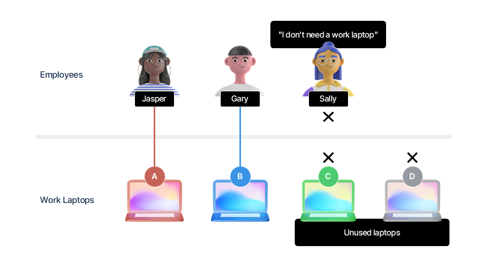
Let’s illustrate the relationship between employees and laptops using tables.
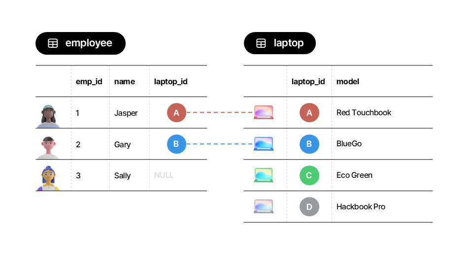
▶️ Create df_employees and df_laptops.
df_employees = pd.DataFrame(
    {
        "emp_id": [1, 2, 3],
        "name": ["Jasper", "Gary", "Sally"],
        "laptop_id": ["A", "B", np.nan],
    }
)

df_employeesdf_laptops = pd.DataFrame(
{
"laptop_id": ["A", "B", "C", "D"],
"model": ["Red Touchbook", "BlueGo", "Eco Green", "Hackbook Pro"],
}
)
df_laptops🔗 Inner Merge (how="inner")
An inner merge is the most common type of join. It returns only the rows where the key ("laptop_id" in our case) exists in both DataFrames. Think of it as the “intersection” of your two tables.
Rule: Only keep rows where there is a match between the two tables.
Here is an illustration of how the inner merge works:
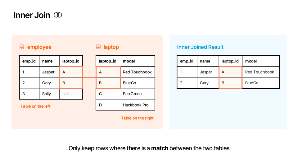
▶️ Perform an inner merge between df_employees and df_laptops on the "laptop_id" column.
df_inner = pd.merge(left=df_employees, right=df_laptops, on="laptop_id", how="inner")

df_inner⬅️ Left Merge (how="left")
A left merge (or left join) keeps every row from the left DataFrame (df_employees). It then brings in matching values from the right DataFrame. If a row from the left DataFrame has no match in the right one, the columns from the right DataFrame are filled with NaN (Not a Number).
Rule: Keep all rows in the left table regardless of matching rows.
Here is an illustration of how the left merge works:
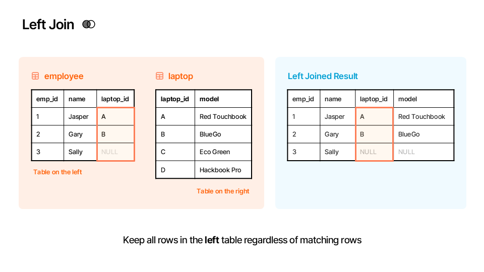
▶️ Perform a left merge between df_employees and df_laptops on the "laptop_id" column.
df_left = pd.merge(left=df_employees, right=df_laptops, on="laptop_id", how="left")

df_left➡️ Right Merge (how="right")
A right merge (or right join) is the opposite of a left merge. It keeps every row from the right DataFrame (df_laptops) and brings in matching values from the left. If a row from the right DataFrame has no match, the columns from the left DataFrame are filled with NaN.
Rule: Keep all rows in the right table regardless of matching rows.
Here is an illustration of how the right merge works:
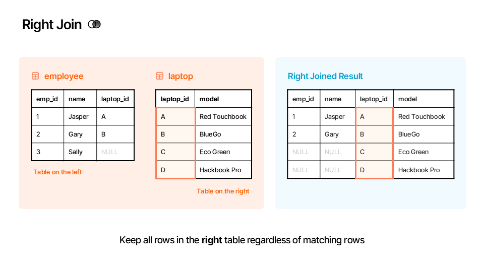
▶️ Perform a right merge between df_employees and df_laptops on the "laptop_id" column.
df_right = pd.merge(left=df_employees, right=df_laptops, on="laptop_id", how="right")

df_right🌐 Outer Merge (how="outer")
A full outer merge (or full outer join) combines the results of both a left and a right merge. It keeps all rows from both DataFrames. Where there isn’t a match, it fills the missing data with NaN. Think of this as the “union” of your two tables.
Rule: Keep all rows from both tables.
Here is an illustration of how the outer merge works:
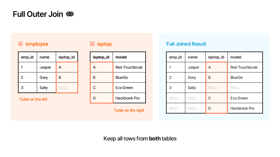
▶️ Perform an outer merge between df_employees and df_laptops on the "laptop_id" column.
df_outer = pd.merge(left=df_employees, right=df_laptops, on="laptop_id", how="outer")

df_outer