Pandas Filtering and Sorting

Import pandas and numpy to follow along with the examples in this page.

import pandas as pd
import numpy as np

🧮 Filtering a `Series`¶

To filter rows in a DataFrame or Series, we can use boolean indexing. This involves creating a boolean mask that indicates which rows meet a certain condition, and then using that mask to select the desired rows.

Boolean indexing can be applied to both DataFrame and Series objects in pandas. This is a powerful and flexible technique for filtering data based on specific criteria.

We’ll start with a simple example using a Series.

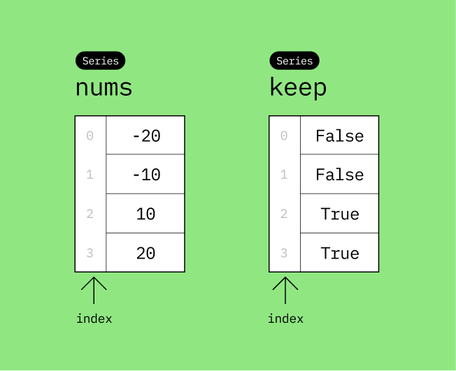
▶️ Create a Series named nums with the following four integers: -20, -10, 10, 20.

nums = pd.Series([-20, -10, 10, 20])

display(nums)

0   -20
1   -10
2    10
3    20
dtype: int64

👉 Our goal is to filter the Series so that it only contains positive values. We’ll first manually create a boolean mask that indicates which values are positive.

▶️ Create a new Series named keep with the following four boolean values: False, False, True, True.

keep = pd.Series([False, False, True, True])

display(keep)

0    False
1    False
2     True
3     True
dtype: bool

Let’s visualize the two Series (nums and keep) you’ve created.

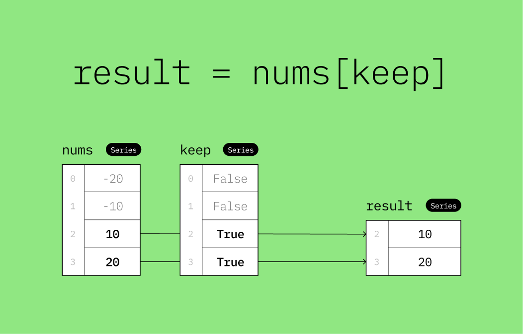
Once we have a boolean mask (the keep Series), we can use it to filter the original Series (nums).

nums[keep]

2    10
3    20
dtype: int64

This can be confusing at first, but the idea is that the True values in the keep Series indicate which values in the nums Series should be kept. The False values indicate which values should be discarded. This is done by passing the keep Series inside the square brackets of the nums Series, like this: nums[keep].

This is called boolean indexing, and it’s a powerful way to filter data in pandas. The boolean Series is a boolean mask that tells pandas which values to keep and which to discard.

If you’re confused about what just happened, this visualization may give you a better idea.

Same Length Requirement

When using boolean indexing, make sure the boolean mask (keep) has the same length as the original Series (nums). Otherwise, you’ll encounter an error.

For example, if keep has fewer elements than nums, you’ll get an IndexingError. In the example below, keep_incorrect has only three boolean values, while nums has four integers. This raises an IndexingError.

⛔️ Heads-up: The code below will throw an error.

nums = pd.Series([-20, -10, 10, 20])
keep_incorrect = pd.Series([False, False, True])
nums[keep_incorrect]
# IndexingError: Unalignable boolean Series provided as indexer

🗂️ Creating Boolean Masks Programmatically¶

The previous example was a bit contrived. We manually created a boolean mask (keep) to filter the nums Series. This is not how you would do it in practice. If you had a Series with millions of elements, you wouldn’t want to manually create a boolean mask with millions of True and False values.

Is there a way to create the boolean mask programmatically? Yes! You can use comparison operators to create boolean masks.

keep_by_comparison = nums > 0

keep_by_comparison

0    False
1    False
2     True
3     True
dtype: bool

The expression nums > 0 compares each element in the nums Series to 0, returning a new boolean Series where each value indicates whether the corresponding value in nums is greater than 0.

You can use other comparison operators as well, such as <, <=, >=, ==, and !=.

The resulting boolean Series is identical to the manually created keep Series from earlier. We can check this using the pd.testing.assert_series_equal() function, which raises an error if the two Series are not equal.

# Manually created boolean mask
display(keep)

# Programmatically created boolean mask
display(keep_by_comparison)

# Check that both boolean masks are identical
pd.testing.assert_series_equal(keep, keep_by_comparison)

0    False
1    False
2     True
3     True
dtype: bool

0    False
1    False
2     True
3     True
dtype: bool

We can use the keep_by_comparison to filter positive values in nums. This works the same way as before where the True values in the boolean mask indicate which values to keep. False values indicate which values to discard.

nums[keep_by_comparison]

2    10
3    20
dtype: int64

Boolean Indexing Does Not Modify Original Data

Filtering elements using a boolean mask returns a new Series without modifying the original Series.

print("Negative Values (filtered):")
display(nums[nums < 10])

# Output:
# Negative Values (filtered):
# 0   -20
# 1   -10
# dtype: int64

print("\n\nOriginal Values:")
display(nums)

# Output:
# Original Values:
# 0   -20
# 1   -10
# 2    10
# 3    20
# dtype: int64

Notice how the original nums Series remains unchanged after filtering.

🎯 Example: Filter even numbers

all_nums = pd.Series([2, 5, 4, 8, -2, -5, -11, 13, 4])

even_nums = all_nums[all_nums % 2 == 0]

even_nums

0    2
2    4
3    8
4   -2
8    4
dtype: int64

🧩 Filtering a `DataFrame`¶

Recall that a DataFrame is a collection of one or more columns, where each column is a Series. This means that filtering a DataFrame is very similar to filtering a Series.

We’ll start by creating a simple DataFrame that contains a list of transactions.

df = pd.DataFrame(
    {"name": ["John", "Mary", "Tom", "John"], "amount": [-20, -10, 10, 20]}
)

display(df)

Assume we want to filter the DataFrame so that it only contains transactions made by "John". There are two transactions made by "John". We can do this by manually creating a boolean mask that indicates which rows have the "name" equal to "John".

is_john = pd.Series([True, False, False, True])

is_john

0     True
1    False
2    False
3     True
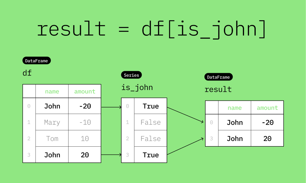
dtype: bool

As before, the True values in the boolean mask indicate which rows to keep. The False values indicate which rows to discard. This is done by passing the boolean mask inside the square brackets of the DataFrame, like this: df[is_john].

result = df[is_john]

result

The visualization below illustrates how df[is_john] works.

🎯 Example: Find all positive transactions programmatically

df = pd.DataFrame(
    {"name": ["John", "Mary", "Tom", "John"], "amount": [-20, -10, 10, 20]}
)
df

To only keep rows where the transaction amount was positive, we can programmatically create a boolean mask that indicates which rows have the amount greater than 0. We can then use this boolean mask to filter the DataFrame.

df_pos = df[df["amount"] > 0]

df_pos

What does df["amount"] > 0 do?

The expression df["amount"] > 0 compares each element in the amount column of the DataFrame to 0, returning a new boolean Series where each value indicates whether the corresponding value in the amount column is greater than 0.

Recall that a column in a DataFrame is a Series. So df["amount"] returns the amount column as a Series. The comparison operator > is then applied element-wise to each value in the amount Series.

This is similar to how we created a boolean mask for the nums Series earlier. Here is the code again for reference:

# Create the nums Series
nums = pd.Series([-20, -10, 10, 20])
# Create a boolean mask to keep only positive values
keep_by_comparison = nums > 0

# Create the DataFrame with transactions
df = pd.DataFrame(
    {"name": ["John", "Mary", "Tom", "John"], "amount": [-20, -10, 10, 20]}
)
# Create a boolean mask to keep only positive transactions
keep_positive_transactions = df["amount"] > 0

⚙️ Logical Operators in `pandas`¶

Pandas supports logical operations on boolean Series. This allows you to combine multiple conditions to create more complex boolean masks.

There are three logical operations you can perform on boolean Series:

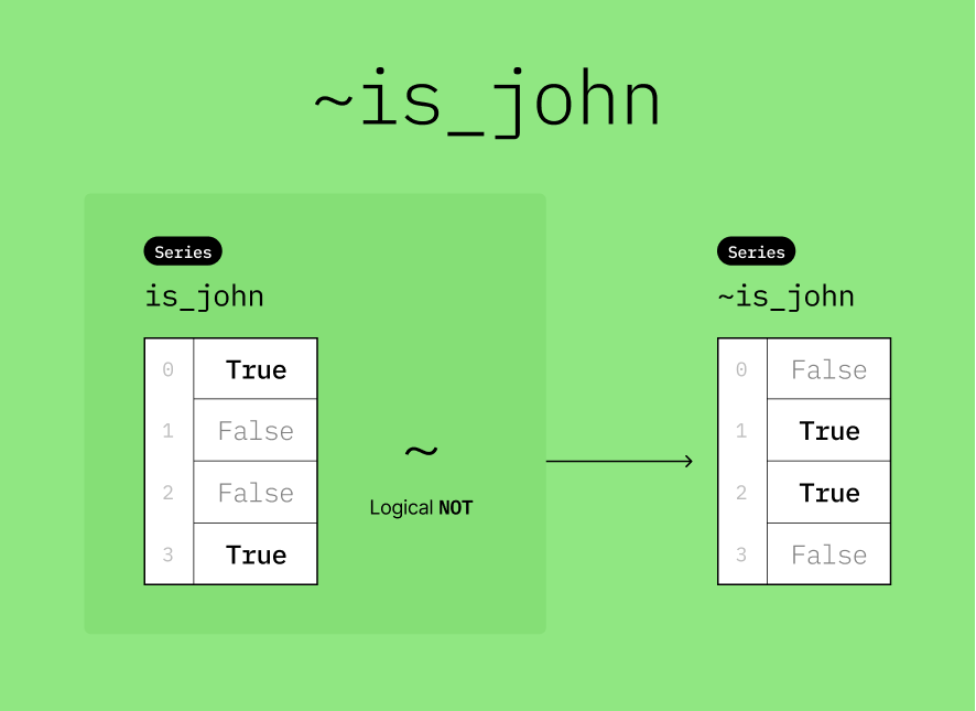
&: Logical AND
|: Logical OR
~: Logical NOT

These operators perform element-wise logical operations on the boolean Series.

For more examples, you can refer to the Pandas documentation on indexing and selecting data.

🤝 Logical AND¶

A logical AND operator & returns True only if both the operands are True.

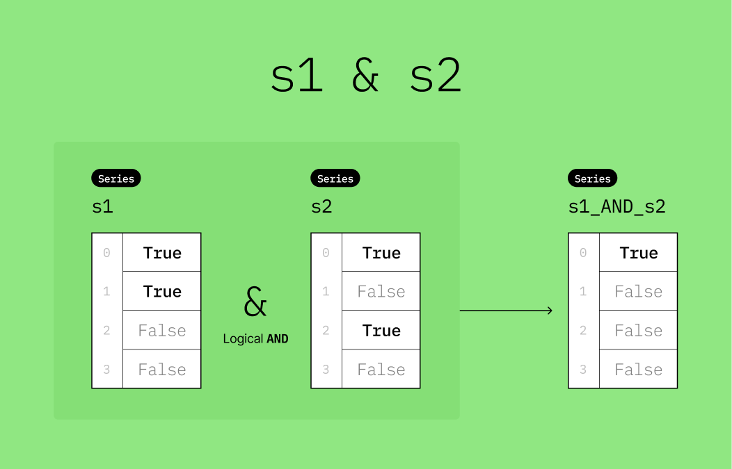
▶️ Perform a logical AND operation (&) on s1 and s2 and store the result to a new variable named s1_AND_s2.

s1 = pd.Series([True, True, False, False])
s2 = pd.Series([True, False, True, False])

s1_AND_s2 = s1 & s2
s1_AND_s2

0     True
1    False
2    False
3    False
dtype: bool

# Display s1, s2, s1_AND_S2 together as a DataFrame
pd.DataFrame({"s1": s1, "s2": s2, "s1_AND_s2": s1_AND_s2})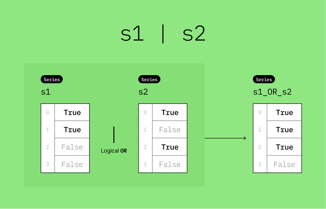

📍 Logical OR¶

A logical OR operator | returns True if either of the operands is True.

▶️ Perform a logical OR operation (|) on s1 and s2 and store the result to a new variable named s1_OR_s2.

s1 = pd.Series([True, True, False, False])
s2 = pd.Series([True, False, True, False])

s1_OR_s2 = s1 | s2
s1_OR_s2

0     True
1     True
2     True
3    False
dtype: bool

# Display s1, s2, s1_OR_s2 together as a DataFrame
pd.DataFrame({"s1": s1, "s2": s2, "s1_OR_s2": s1_OR_s2})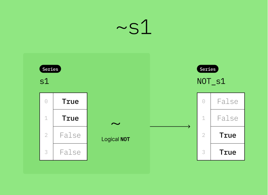

❗ Logical NOT¶

A logical NOT operator ~ reverses each operand.

▶️ Perform a logical OR operation (~) on s1 and store the result to a new variable named NOT_s1.

s1 = pd.Series([True, True, False, False])

NOT_s1 = ~s1
NOT_s1

0    False
1    False
2     True
3     True
dtype: bool

# Display s1 and NOT_s1 together as a DataFrame
pd.DataFrame({"s1": s1, "NOT_s1": NOT_s1})

✅ Putting It All Together¶

Here is a summary of the logical operations you’ve performed so far.

pd.DataFrame(
    {"s1": s1, "s2": s2, "s1_AND_s2": s1_AND_s2, "s1_OR_s2": s1_OR_s2, "NOT_s1": NOT_s1}
)

🎯 Example: Find John’s positive transaction(s)

# DO NOT CHANGE THE CODE IN THIS CELL
df = pd.DataFrame(
    {"name": ["John", "Mary", "Tom", "John"], "amount": [-20, -10, 10, 20]}
)

# Create two boolean masks
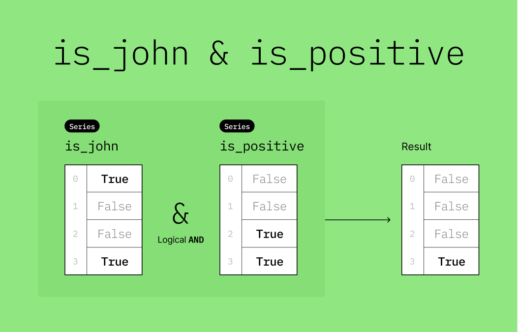
is_john = df["name"] == "John"
is_positive = df["amount"] > 0

# Apply both conditions using the & operator
df_john_and_pos = df[is_john & is_positive]

df_john_and_pos

What do is_john and is_positive represent?

is_john is a boolean mask that indicates which rows in the DataFrame have the name “John”.
is_positive is a boolean mask that indicates which rows in the DataFrame have a positive amount.

is_john
display(is_john)

# Output:
# 0     True
# 1    False
# 2    False
# 3     True
# Name: name, dtype: bool

is_positive
display(is_positive)
# Output:
# 0    False
# 1    False
# 2     True
# 3     True
# Name: amount, dtype: bool

Here’s a visualization to help you understand what is_john & is_positive does.

🎯 Example: Find transactions that are made by John OR are positive

# DO NOT CHANGE THE CODE IN THIS CELL
df = pd.DataFrame(
    {"name": ["John", "Mary", "Tom", "John"], "amount": [-20, -10, 10, 20]}
)
df

df = pd.DataFrame(
    {"name": ["John", "Mary", "Tom", "John"], "amount": [-20, -10, 10, 20]}
)

# Create two boolean masks
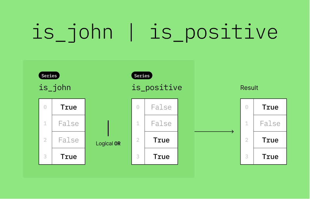
is_john = df["name"] == "John"
is_positive = df["amount"] > 0

# Apply either condition using the | operator
df_john_or_pos = df[is_john | is_positive]

df_john_or_pos

Here is a visualization to help you understand what is_john | is_positive does.

🎯 Example: Find transactions that are NOT made by John

df = pd.DataFrame(
    {"name": ["John", "Mary", "Tom", "John"], "amount": [-20, -10, 10, 20]}
)

# Create a boolean mask where the name is "John"
is_john = df["name"] == "John"

# Create a boolean mask with the NOT operator
# This will effectively select rows where the name is NOT "John"
df_not_john = df[~is_john]

df_not_john

Here’s a visualization to help you understand what ~is_john does.

🗣️ String Comparison on a `Series`¶

Create a new Series named countries.

countries = pd.Series(
    ["United States", "Oman", "United States", "China", "South Korea", "United States"]
)

display(countries)

0    United States
1             Oman
2    United States
3            China
4      South Korea
5    United States
dtype: object

We can perform element-wise comparisons on string Series just like we did with numeric Series.

▶️ Compare countries with the string "United States" using an equality comparison operator (==).

countries == "United States"

0     True
1    False
2     True
3    False
4    False
5     True
dtype: bool

▶️ Check the data type of the result.

type(countries == "United States")

pandas.core.series.Series

The result is another Series containing boolean (True/False) values. Pandas performs a string comparison (my_str == "United States") on each element.

Remember, you can also supply more than one condition using the following two operators:

logical OR (|)
logical AND (&)

▶️ Check whether a country is either "Oman" or "China".

(countries == "Oman") | (countries == "China")

0    False
1     True
2    False
3     True
4    False
5    False
dtype: bool

We can use the resulting boolean Series as a mask to filter the original countries Series.

countries[(countries == "Oman") | (countries == "China")]

1     Oman
3    China
dtype: object

🔤 Applying a Mask to a `DataFrame`¶

Create a new DataFrame named df_cities.

df_cities = pd.DataFrame(
    {
        "city": ["Lisle", "Dubai", "Niles", "Shanghai", "Seoul", "Chicago"],
        "country": [
            "United States",
            "United Arab Emirates",
            "United States",
            "China",
            "South Korea",
            "United States",
        ],
        "population": [23270, 3331409, 28938, 26320000, 21794000, 8604203],
    }
)

df_cities

To only keep rows where the country is "United States", we can supply a Series of boolean values.

Create a new Series named keep with the following 6 boolean values - True, False, True, False, False, True.

# Manually (not recommended)
keep = pd.Series([True, False, True, False, False, True])

# Programmatically (preferred)
keep = df_cities["country"] == "United States"

keep

0     True
1    False
2     True
3    False
4    False
5     True
Name: country, dtype: bool

To only keep rows where the "country" is "United States", use the boolean mask keep to filter the df_cities DataFrame.

df_cities[keep]

🎯 Example: Cities with population over a million

df_large_cities = df_cities[df_cities["population"] > 1000000]

df_large_cities

🆙 Sorting a `DataFrame`¶

You can sort a DataFrame using df.sort_values().

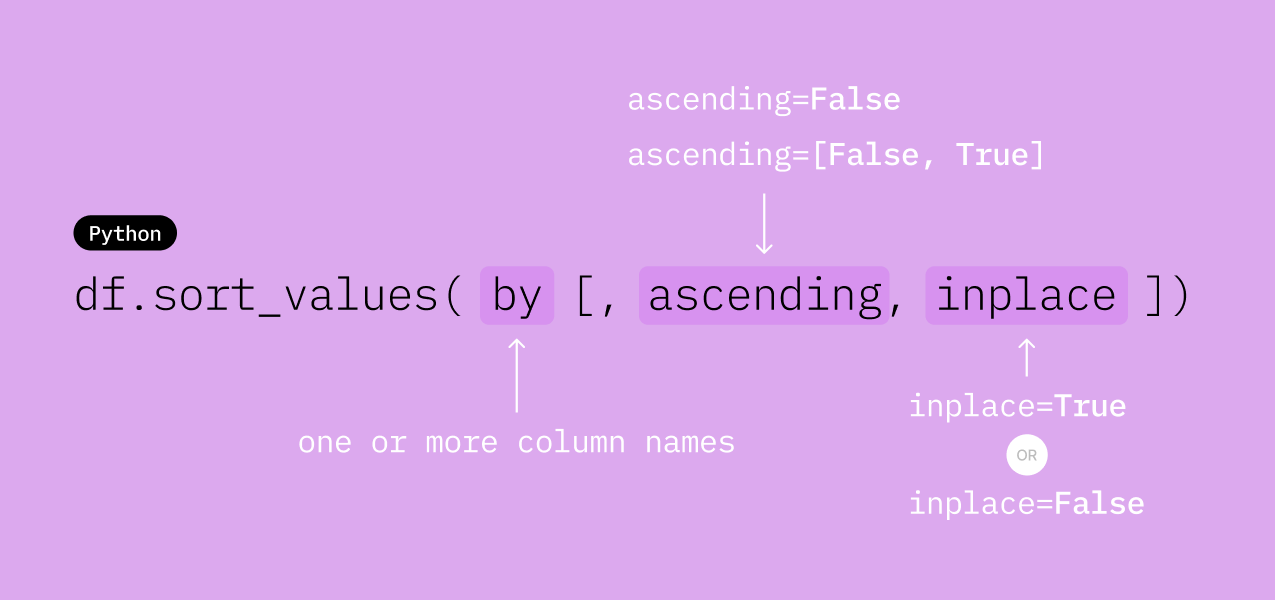
The sort() method allows you to specify the column(s) to sort by, the sorting order (ascending or descending), and how to handle missing values.

The by parameter specifies the column(s) to sort by. You can pass a single column name as a string or multiple column names as a list of strings.

The ascending parameter specifies the sorting order. By default, it is set to True, which means the data will be sorted in ascending order. If you want to sort in descending order, you can set this parameter to False.

If there are multiple columns specified in the by parameter, you can pass a list of boolean values to the ascending parameter to specify the sorting order for each column individually.

If there are missing values (NaN) in the column(s) being sorted, you can use the na_position parameter to specify whether to place them at the beginning ("first") or the end ("last") of the sorted DataFrame. The default is "last".

▶️ Sort df_cities by "population".

df_cities.sort_values("population")

▶️ Sort df_cities by "population" in descending order.

df_cities.sort_values("population", ascending=False)

👟 Examples using the Yeezys Dataset¶

df_sneakers = pd.read_csv(
    "https://github.com/bdi475/datasets/raw/main/yeezy_sneakers.csv"
)

# head() displays the first 5 rows of a DataFrame
df_sneakers.head()

The table below describes the columns in df_sneakers.

Column Name	Description
brand	Brand of the sneaker
product	Name of the sneaker
price	Price of the sneaker

▶️ Print out a summary of the df_sneakers using the info() method.

df_sneakers.info()

<class 'pandas.core.frame.DataFrame'>
RangeIndex: 15 entries, 0 to 14
Data columns (total 3 columns):
 #   Column   Non-Null Count  Dtype 
---  ------   --------------  ----- 
 0   brand    15 non-null     object
 1   product  15 non-null     object
 2   price    15 non-null     int64 
dtypes: int64(1), object(2)
memory usage: 492.0+ bytes

The .shape attribute returns a tuple representing the dimensionality of the DataFrame. The first element is the number of rows, and the second element is the number of columns.

▶️ Use df_sneakers.shape to see the shape of the DataFrame.

df_sneakers.shape

(15, 3)

We can retrieve the number of rows and columns separately by indexing into the tuple returned by the .shape attribute.

num_rows = df_sneakers.shape[0]
num_cols = df_sneakers.shape[1]

print(f"Number of rows: {num_rows}")
print(f"Number of columns: {num_cols}")

Number of rows: 15
Number of columns: 3

Alternatively, you can unpack the tuple returned by .shape into two separate variables. This is called tuple unpacking or destructuring assignment.

num_rows, num_cols = df_sneakers.shape

print(f"Number of rows: {num_rows}")
print(f"Number of columns: {num_cols}")

Number of rows: 15
Number of columns: 3

🎯 Example: Find "Adidas" sneakers

df_adidas = df_sneakers[df_sneakers["brand"] == "Adidas"]

df_adidas

🎯 Example: Find Sneakers under \$1,000

df_under_1000 = df_sneakers[df_sneakers["price"] < 1000]

df_under_1000

🎯 Example: Find "Nike" Sneakers over \$3,000

df_nike_over_3000 = df_sneakers[
    (df_sneakers["brand"] == "Nike") & (df_sneakers["price"] > 3000)
]

df_nike_over_3000

Why the parentheses?

In the code above, we used parentheses to group the conditions inside the query method:

df_sneakers[
    (df_sneakers["brand"] == "Nike") & (df_sneakers["price"] > 3000)
]

The parentheses are used to group the conditions in the query method. This ensures that the filtering is applied correctly, first checking for the brand and then for the price.

Without the parentheses, the logical operators & (AND) and | (OR) have higher precedence than comparison operators like == and >. This means that without parentheses, the expression would first attempt to evaluate "Nike" & df_sneakers["price"], which is not a valid operation and would raise a TypeError.

df_sneakers[
    df_sneakers["brand"] == "Nike" & df_sneakers["price"] > 3000
]
# TypeError: Cannot perform 'rand_' with
# a dtyped [int64] array and scalar of type [bool]

🎯 Example: Sort sneakers by price in descending order

df_sorted_by_price_desc = df_sneakers.sort_values("price", ascending=False)

df_sorted_by_price_desc

🎯 Example: Sneakers > 6000 or < 1000

df_polar = df_sneakers[(df_sneakers["price"] > 6000) | (df_sneakers["price"] < 1000)]

df_polar

🎯 Example: Sort by brand ascending and price descending

df_sorted_by_brand_price = df_sneakers.sort_values(
    ["brand", "price"], ascending=[True, False]
)

df_sorted_by_brand_price

Can I use .sort_values() twice instead of passing a list to by?

No, you cannot use .sort_values() twice to achieve the same result as passing a list to the by parameter. When you call .sort_values() multiple times, each call sorts the entire DataFrame independently, which means the second sort will override the first sort.

For example, the following code will not sort df_sneakers first by "brand". The second .sort_values() call will then sort by "price". Note that the final result will only be sorted by "price" in descending order, and the sorting by "brand" will be lost. If you’re looking to sort by multiple columns, you should pass a list of column names to the by parameter in a single .sort_values() call.

🚫 Incorrect approach: Call sort_values() separately

In this approach, we first sort by "brand" and then by "price", but the second sort overrides the first. df_temporary is an intermediate DataFrame that holds the result of the first sort. The final result, df_sorted_by_brand_price, is only sorted by "price" in descending order.

df_temporary = df_sneakers.sort_values("brand", ascending=True)
df_sorted_by_brand_price = df_temporary.sort_values("price", ascending=False) # Not correct

✅ Correct approach: Pass a list to by

df_sorted_by_brand_price = df_sneakers.sort_values(
    ["brand", "price"], ascending=[True, False]
)

The code and output below verify that the result is only sorted by "price" in descending order, and the sorting by "brand" is lost.

df_chained_sort = df_sneakers.sort_values("brand", ascending=True).sort_values(
    "price", ascending=False
)

df_chained_sort

🧑‍💼 More Examples using an Employees `DataFrame`¶

Create a new DataFrame named df_emp.

df_emp = pd.DataFrame(
    {
        "emp_id": [30, 40, 10, 20],
        "name": ["Colby", "Adam", "Eli", "Dylan"],
        "dept": ["Sales", "Marketing", "Sales", "Marketing"],
        "office_phone": ["(217)123-4500", np.nan, np.nan, "(217)987-6543"],
        "start_date": ["2017-05-01", "2018-02-01", "2020-08-01", "2019-12-01"],
        "salary": [202000, 185000, 240000, 160500],
    }
)

# Used for intermediate checks
df_emp_backup = df_emp.copy()

df_emp

🎯 Example: Sort by "emp_id" ascending

df_id_asc = df_emp.sort_values("emp_id")

df_id_asc

🎯 Example: Sort by "emp_id" descending

df_id_desc = df_emp.sort_values("emp_id", ascending=False)

df_id_desc

🎯 Example: Sort by "dept" descending and then by "start_date" ascending

df_dept_desc_date_asc = df_emp.sort_values(
    ["dept", "start_date"], ascending=[False, True]
)

df_dept_desc_date_asc

🎯 Example: Sort by "dept" ascending and then by "salary" descending

df_dept_asc_salary_desc = df_emp.sort_values(
    ["dept", "salary"], ascending=[True, False]
)

df_dept_asc_salary_desc

🔄 In-place vs Out-of-place Sorting¶

When you sort a DataFrame using the sort_values() method, you have the option to sort the data in-place or to create a new sorted DataFrame.

An in-place sort modifies the original DataFrame, while an out-of-place sort returns a new sorted DataFrame without modifying the original.

In-place sorting is done by setting the inplace parameter to True. By default, inplace is set to False, which means the original DataFrame remains unchanged and a new sorted DataFrame is returned.

Here’s an example of out-of-place sorting (the default behavior):

df_sorted = df.sort_values("column_name", ascending=False)

df remains unchanged after this operation. The assignment operation creates a new variable named df_sorted that contains the sorted data.

Here’s an example of in-place sorting:

df.sort_values("column_name", inplace=True)

This directly modifies df, and there is no need to assign the result to a new variable. After this operation, df will be sorted.

Common Mistake: Using an Assignment with In-place Sorting

When using in-place sorting (inplace=True), the method does not return a new DataFrame. Therefore, if you try to assign the result of an in-place sort to a new variable, that variable will be set to None.

This is a common mistake. For example, the following code will set df_sorted to None because sort_values() does not return anything when inplace=True.

🚫 Incorrect approach: Use an assignment with in-place sorting

df_sorted = df.sort_values("column_name", inplace=True)
display(df_sorted)  # Output: None

✅ Correct approach: Do not use an assignment with in-place sorting

df.sort_values("column_name", inplace=True)
display(df)  # Output: Sorted DataFrame

🎯 Example: Sort by "salary" descending in-place

df_emp.sort_values("salary", ascending=False, inplace=True)

df_emp

🎯 Example: Sort by "department" and "name" both descending in-place

df_emp.sort_values(["dept", "name"], ascending=[False, False], inplace=True)

df_emp

💾 Writing a `DataFrame` to a CSV File¶

You can write a DataFrame to a CSV file using the df.to_csv() method.

df_cities.to_csv("cities.csv", index=False)

This will create a file named cities.csv in the current working directory. The index=False argument is used to prevent pandas from writing row indices to the CSV file.

The resulting CSV file will look like this:

city,country,population
Lisle,United States,23270
Dubai,United Arab Emirates,3331409
Niles,United States,28938
Shanghai,China,26320000
Seoul,South Korea,21794000
Chicago,United States,8604203

You can also write a DataFrame to different file formats, such as Excel, JSON, and SQL databases, using the appropriate pandas methods like to_excel(), to_json(), and to_sql(). For more information, refer to the Pandas documentation on I/O tools.

Tools Used in This Course

Introduction to Pandas

Tools Used in This Course

Pandas Data Types, Column Operations, and Missing Values

🧮 Filtering a Series¶

🗂️ Creating Boolean Masks Programmatically¶

🧩 Filtering a DataFrame¶

⚙️ Logical Operators in pandas¶